Some Machine Learning Methods for NeuroImaging Analysis
Xi (Rossi) LUO
Health Science Center
School of Public Health
Dept of Biostatistics
and Data Science
September 17, 2019
Funding: NIH R01EB022911, P01AA019072, P20GM103645, P30AI042853; NSF/DMS (BD2K) 1557467
Slides viewable on web:
BigComplexData.com
Overall Theme
- Machine learning: develop new models
- Optimization: fast and large-scale computation
- Theory: some theoretic properties
- Neuroimaging: big and complex data
Granger Mediation Analysis
Co-Author
Yi Zhao
Tenure-track Assistant Prof at Indiana Univ
fMRI Experiments
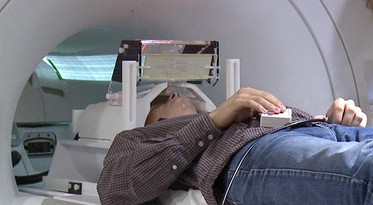
- Task fMRI: performs tasks under brain scanning
-
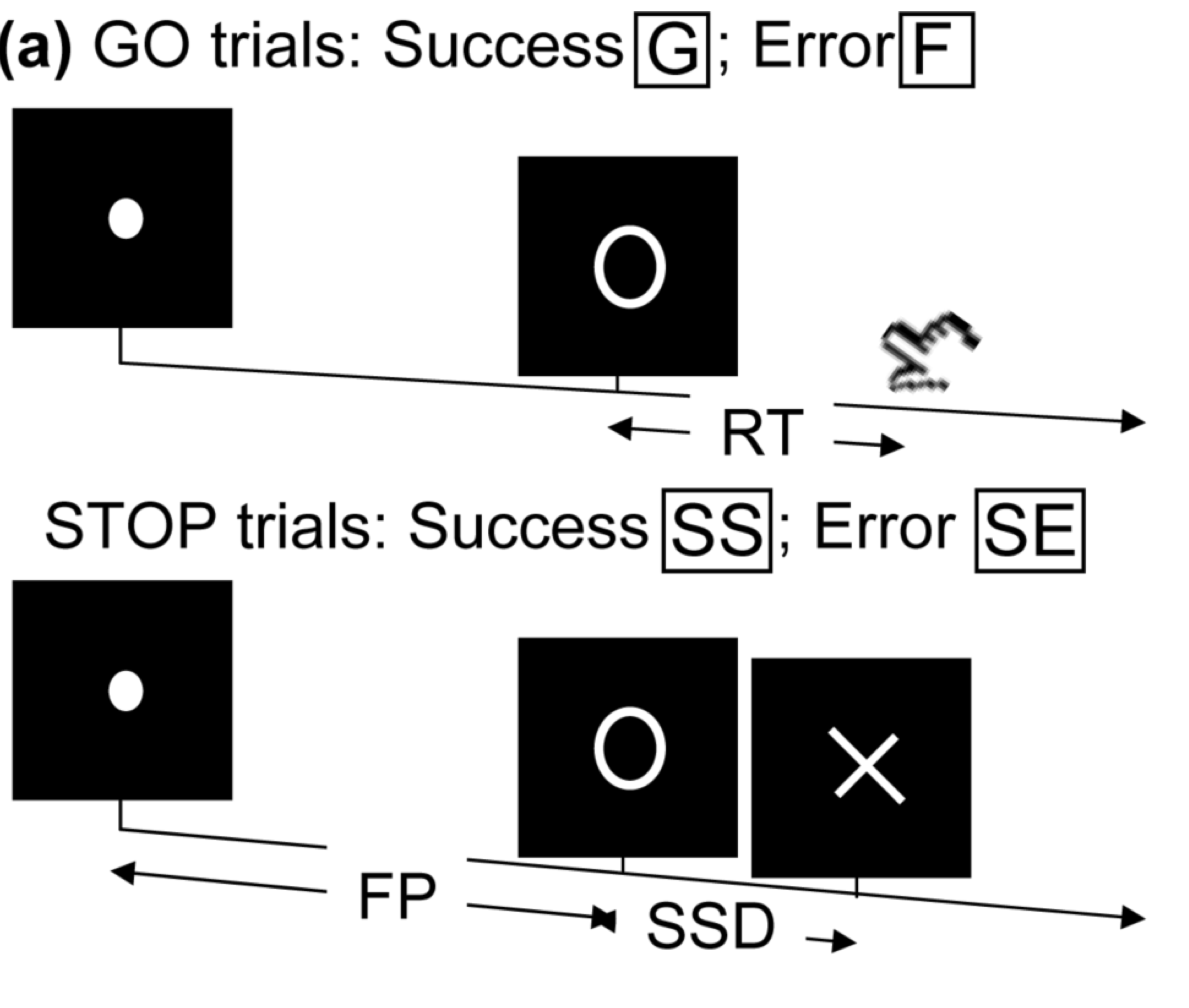
Randomized stop/go task:- press button if "go";
- withhold pressing if "stop"
- Not resting-state: "do nothing" during scanning
fMRI data: blood-oxygen-level dependent (BOLD) signals from each
Multilevel fMRI Studies
Sub 1, Sess 1
Time 1
2
…
~200
⋮
Sub i, Sess j
…
⋮
Sub ~100, Sess ~4
…
e.g. $1000 \times 4 \times 300 \times 10^6 \approx 1 $ trillion data points
Raw Data: Motor Region
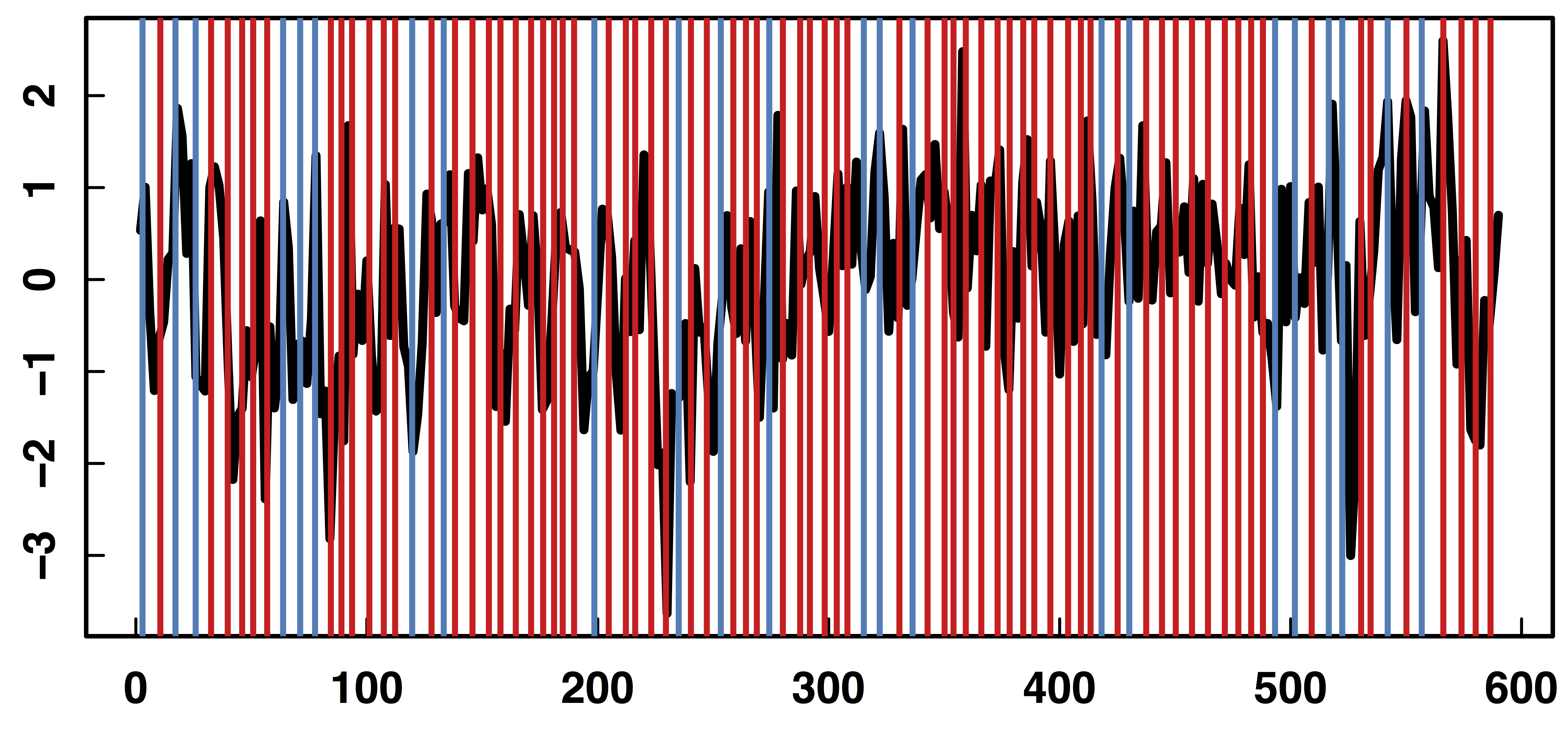
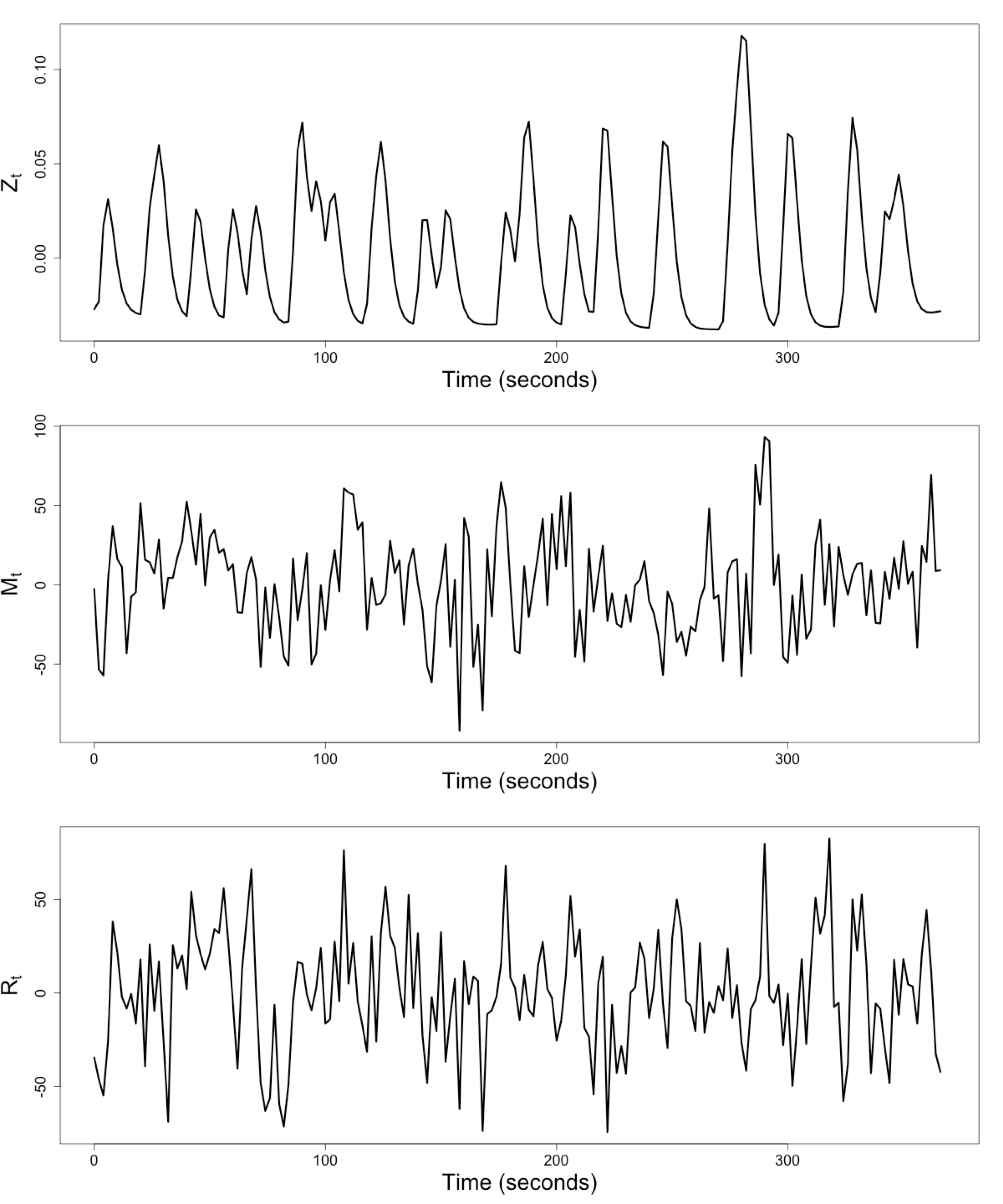
$Z_t$: Stimulus onsets convoluted with Canonical HRF
$M_t$, $R_t$: fMRI time series from two brain regions
Review: Granger Causality/VAR
- Given two (or more) time series $x_t$ and $y_t$ $$\begin{align*} x_t &= \sum_{j=1}^p \psi_{1j} x_{t-j} + \sum_{j=1}^p \phi_{1j} y_{t-j} + \epsilon_{1t} \\ y_t &= \sum_{j=1}^p \psi_{2j} y_{t-j} + \sum_{j=1}^p \phi_{2j} x_{t-j} + \epsilon_{2t} \end{align*}$$
- Also called vector autoregressive models
- $y$ Granger causes $x$ if $\phi_{1j} \ne 0$ Granger, 69
- Models
pair-wise connections notpathways
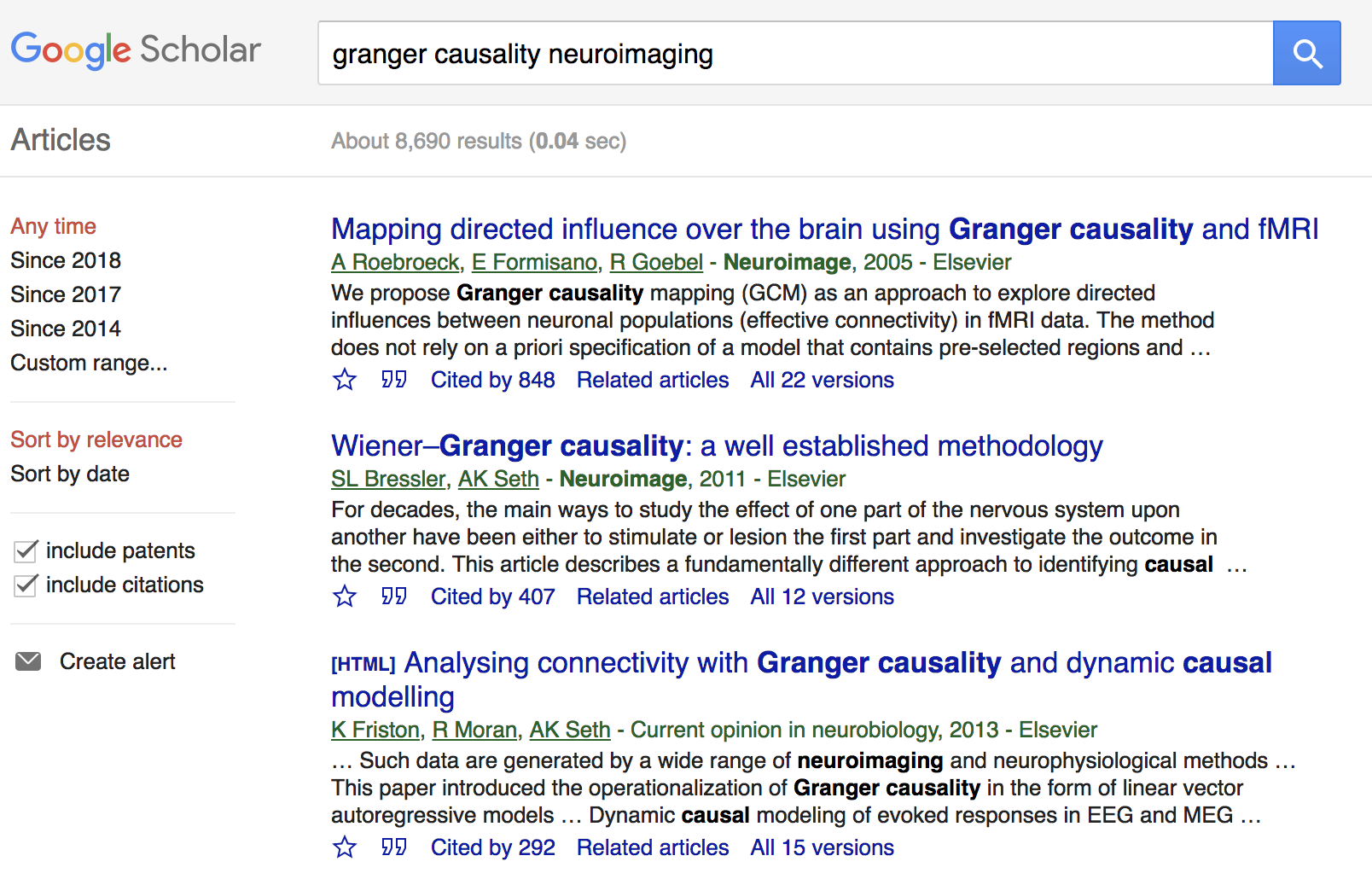
Granger Causality/VAR
- Granger Causality (VAR) popular for fMRI
- Over
10,000 google scholar results on "granger causality neuroimaging", as of May 29, 2019
- Over
- Models multiple
stationary time series - AR($p$) (small $p$) fits fMRI well Lingdquist, 08
Not fornon-stationary /task fMRICannot model stimulus effects
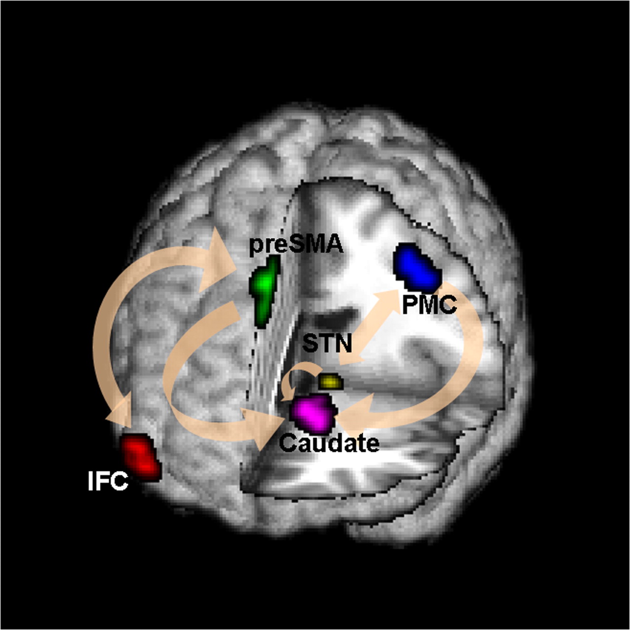
Conceptual Brain Model with Stimulus
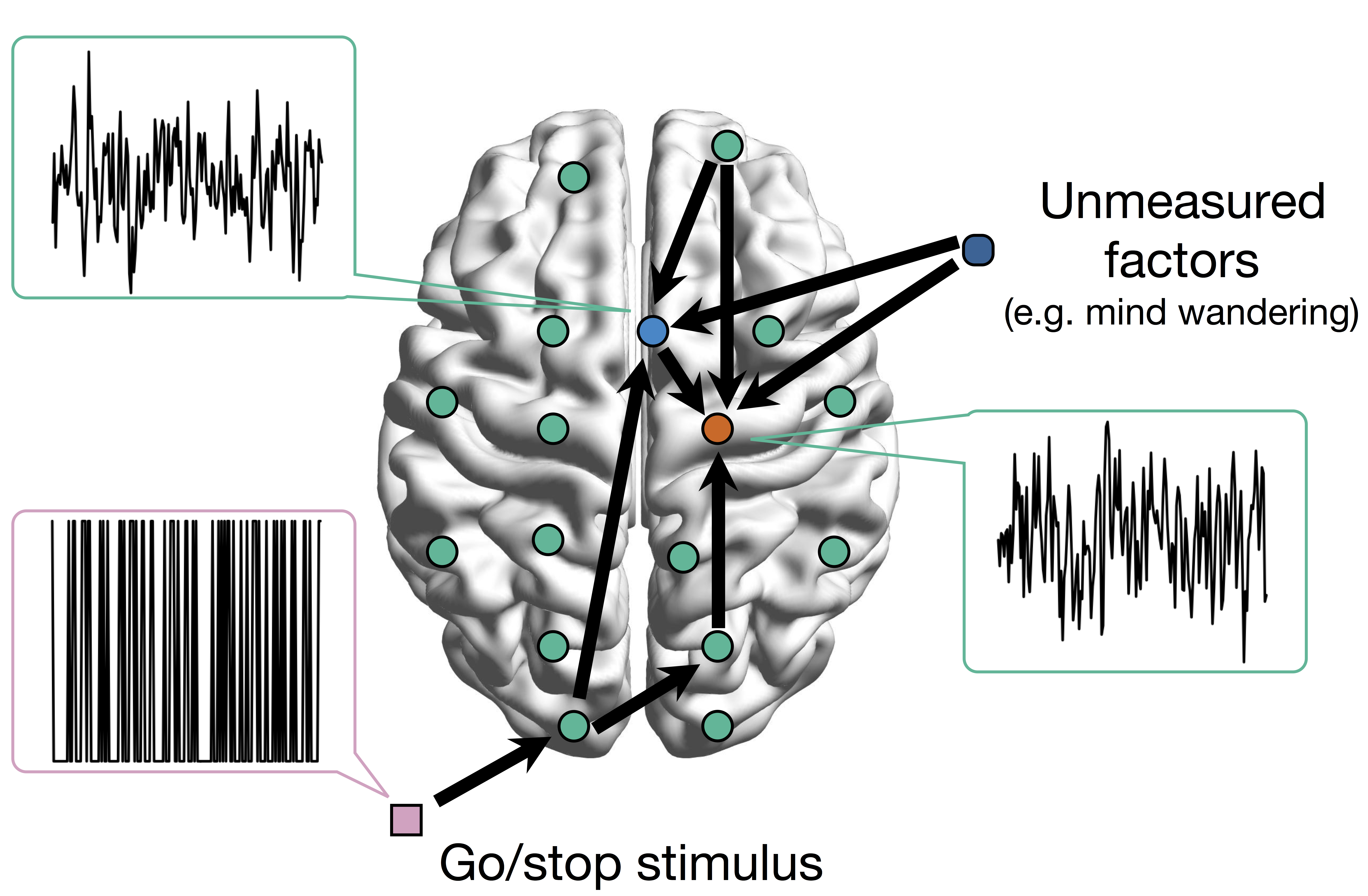
Goal: quantify effects stimuli → preSMA → PMC regions Duann, Ide, Luo, Li (2009). J of Neurosci
Model: Mediation Analysis and SEM
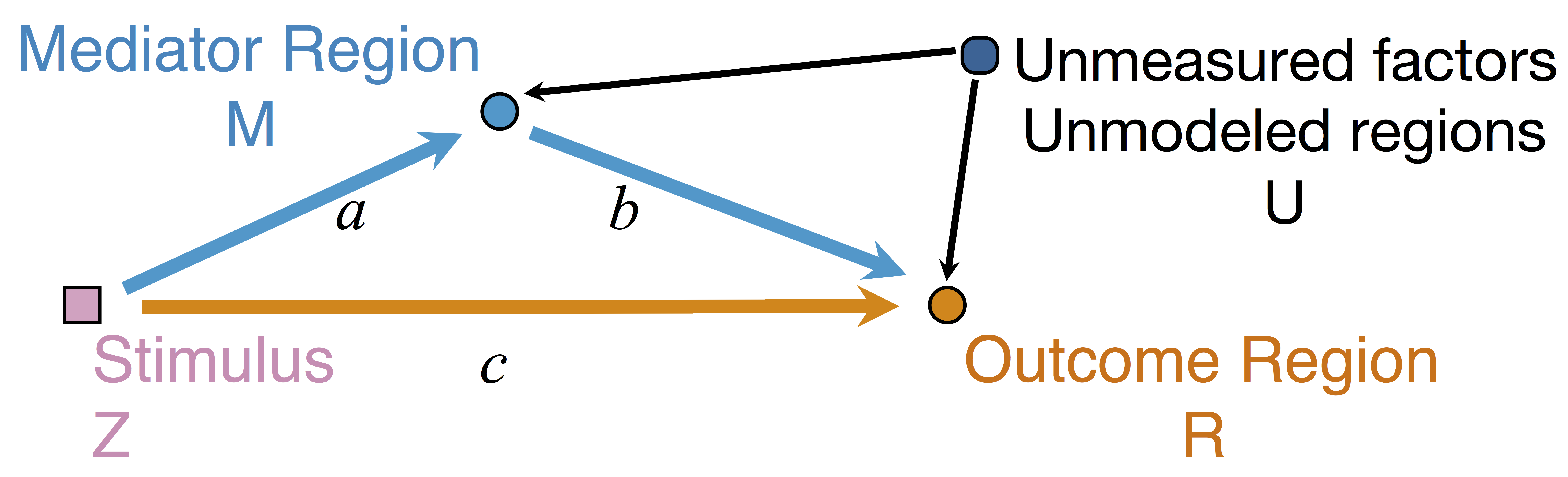 $$\begin{align*}M &= Z a + \overbrace{U + \epsilon_1}^{E_1}\\ R &= Z c + M b + \underbrace{U g + \epsilon_2}_{E_2}, \quad \epsilon_1 \bot \epsilon_2\end{align*}$$
-
Indirect effect: $a \times b$; Direct effect: $c$ - Correlated errors: $\delta = \cor(E_1, E_2) \ne 0$ if $U\ne 0$
Mediation Analysis in fMRI
- Mediation analysis (usually assuming $U=0$)Baron&anp;Kenny, 86; Sobel, 82; Holland 88; Preacher&Hayes 08; Imai et al, 10; VanderWeele, 15;...
- Parametric Wager et al, 09 and functional Lindquist, 12 mediation, under (approx.) independent errors
- Stimulus $\rightarrow$ brain $\rightarrow$
user reported ratings , one brain mediator - Assuming $U=0$ between ratings and brain
- Stimulus $\rightarrow$ brain $\rightarrow$
- Multiple mediator and multiple pathways
- Dimension reduction by arXiv1511.09354Chen, Crainiceanu, Ogburn, Caffo, Wager, Lindquist, 15
- Pathway Lasso penalization Zhao, Luo, 16
- This talk: integrating Granger causality and mediation analysis
Model & Method
Our Mediation Model
$$\begin{align*}M_{t} = Z_{t} a + E_{1t},\quad R_t = Z_t c + M_t b + E_{2t}\end{align*}$$Temporal VAR errors $$\begin{align*} E_{1t}&=& \sum_{j=1}^{p}\left(\omega_{11_{j}}E_{1,t-j}+\omega_{21_{j}}E_{2,t-j}\right)+\epsilon_{1t} \\ E_{2t}&=&\sum_{j=1}^{p}\left(\omega_{12_{j}}E_{1,t-j}+\omega_{22_{j}}E_{2,t-j}\right)+\epsilon_{2t} \end{align*}$$Spatial errors: $\epsilon_{1t}, \epsilon_{2t}$ $$ \begin{pmatrix} \epsilon_{1t} \\ \epsilon_{2t} \end{pmatrix}\sim\mathcal{N}\left(\boldsymbol{\mathrm{0}},\boldsymbol{\Sigma}\right), \quad \boldsymbol{\Sigma}=\begin{pmatrix} \sigma_{1}^{2} & \delta\sigma_{1}\sigma_{2} \\ \delta\sigma_{1}\sigma_{2} & \sigma_{2}^{2} \end{pmatrix} $$
Equivalent Form
$$\begin{align*} \scriptsize M_{t}& \scriptsize =Z_{t}A+\sum_{j=1}^{p}\left(\phi_{1j}Z_{t-j}+\psi_{11_{j}}M_{t-j}+\psi_{21_{j}}R_{t-j}\right)+\epsilon_{1t} \\ \scriptsize R_{t}& \scriptsize =Z_{t}C+M_{t}B+\sum_{j=1}^{p}\left(\phi_{2j}Z_{t-j}+\psi_{12_{j}}M_{t-j}+\psi_{22_{j}}R_{t-j}\right)+\epsilon_{2t} \end{align*} $$- Nonzero $\phi$'s and $\psi$'s denote the temporal influence from stimulus to mediator/outcome and etc
- $A$, $B$, $C$ are causal following a similar proof in Sobel, Lindquist, 04
Causal Conditions
- The treatment randomization regime is the same across time and participants.
- Models are correctly specified, and no treatment-mediator interaction.
- At each time point $t$, the observed outcome is one realization of the potential outcome with observed treatment assignment $\mathbf{\bar S}_{t}$, where $\mathbf{ \bar S}_{t}=( \mathbf{S}_{1},\dots,\mathbf{S}_{t})$.
- The treatment assignment is random across time.
- The causal effects are time-invariant.
- The time-invariant covariance matrix is not affected by the treatment assignments.
Estimation: Conditional Likelihood
- The full likelihood for our model is too complex
- Given the initial $p$ time points, the conditional likelihood is $$ \begin{align*} & \tiny \ell\left(\boldsymbol{\Theta},\delta~|~\mathbf{Z},\mathcal{I}_{p}\right) = \sum_{t=p+1}^{T}\log f\left((M_{t},R_{t})~|~\mathbf{X}_{t}\right) \\ & \tiny = -\frac{T-p}{2}\log\sigma_{1}^{2}\sigma_{2}^{2}(1-\delta^{2})-\frac{1}{2\sigma_{1}^{2}}\|\mathbf{M}-\mathbf{X}\boldsymbol{\theta}_{1}\|_{2}^{2} \\ & \tiny -\frac{1}{2\sigma_{2}^{2}(1-\delta^{2})}\|(\mathbf{R}-\mathbf{M}B-\mathbf{X}\boldsymbol{\theta}_{2})-\kappa(\mathbf{M}-\mathbf{X}\boldsymbol{\theta}_{1})\|_{2}^{2} \end{align*} $$
Multilevel Data: Two-level Likelihood
- Second level model, for each subject $i$ $$(A_i,B_i,C_i) = (A,B,C) + (\eta^A_i, \eta^B_i, \eta^C_i)$$ where errors $\eta$ are normally distributed
- The two level likelihood is conditional convex
- Two-stage fitting: plug-in estimates from the first level
- Block coordinate fitting: jointly optimize first level likelihood + second level likelihood
1. If $\boldsymbol{\Lambda}$ is known, then the two-stage estimator $\hat{\delta}$ maximizes the profile likelihood of model asymptotically, and $\hat{\delta}$ is $\sqrt{NT}$-consistent.
2. If $\boldsymbol{\Lambda}$ is unknown, then the profile likelihood of model has a unique maximizer $\hat{\delta}$ asymptotically, and $\hat{\delta}$ is $\sqrt{NT}$-consistent, provided that $1/\varpi=\bar{\kappa}^{2}/\varrho^{2}=\mathcal{O}_{p}(1/\sqrt{NT})$, $\kappa_{i}=\sigma_{i_{2}}/\sigma_{i_{1}}$, $\bar{\kappa}=(1/N)\sum\kappa_{i}$, and $\varrho^{2}=(1/N)\sum(\kappa_{i}-\bar{\kappa})^{2}$.
Using the two-stage estimator $\hat{\delta}$, the CMLE of our model is consistent, as well as the estimator for $\mathbf{b}=(A,B,C)$.
Theory: Summary
- Under regularity conditions, $N$ subs, $T$ time points
- Our $\hat \delta$ is $\sqrt{NT}$-consistent
- This relaxes the unmeasured confounding assumption in mediation analysis
- Our $(\hat{A},\hat{B}, \hat{C})$ is also consistent
Simulations & Real Data
Comparison
- Our methods:
GMA-h andGMA-ts - Previous methods: BK Baron & Kenny, MACC Zhao and Luo, KKB Kenny et al
- Other methods do not model the temporal correlations or time series like ours
Simulations
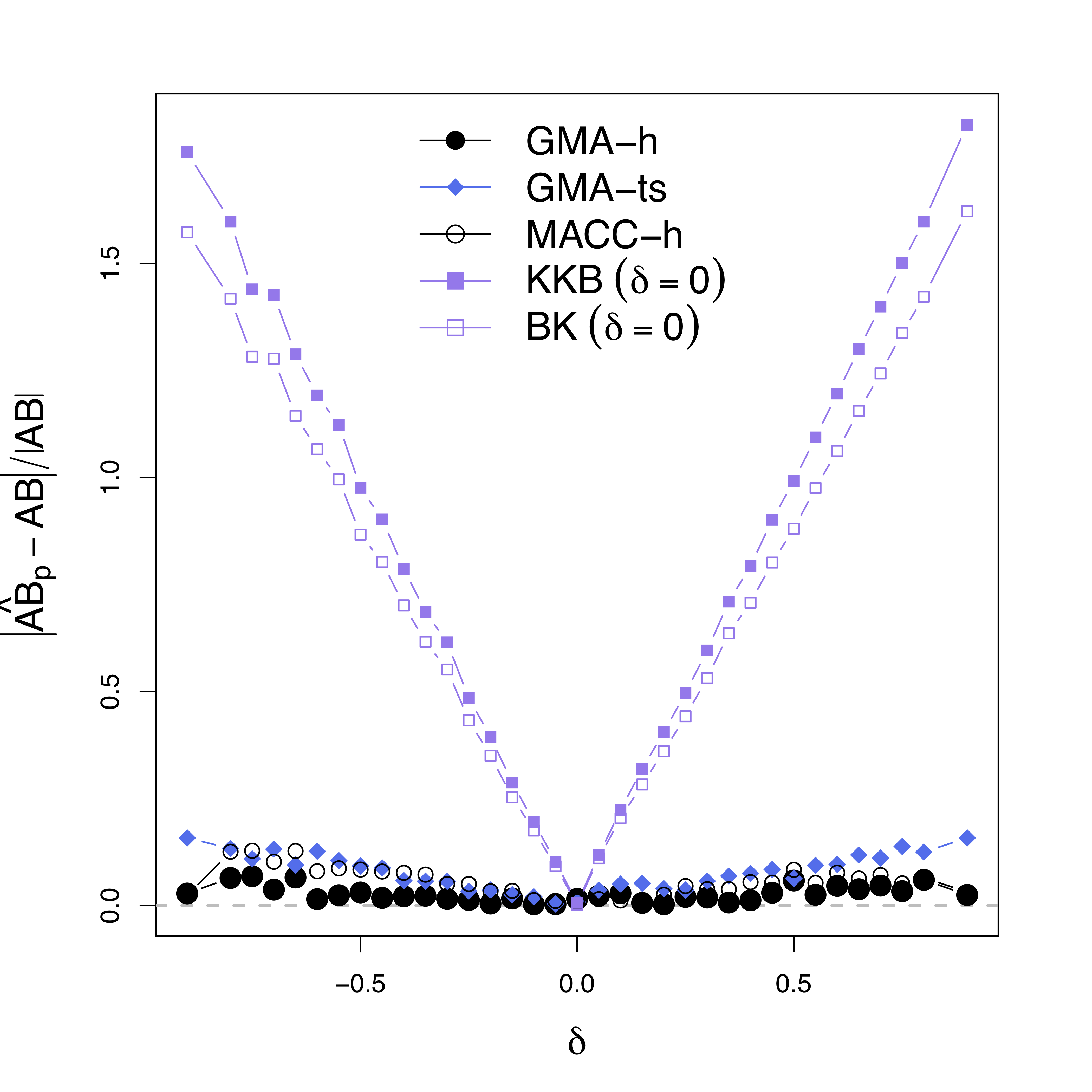
Low bias for $AB$
Low bias for temporal cor
Gray dash lines are the truth
Real Data Experiment
- Public data: OpenFMRI ds30
- Stop-go experiment: withhold (STOP) from pressing buttons
- Expect "STOP" stimuli to deactivate brain region M1
- Goal: quantify the role of region preSMA
Result
Result
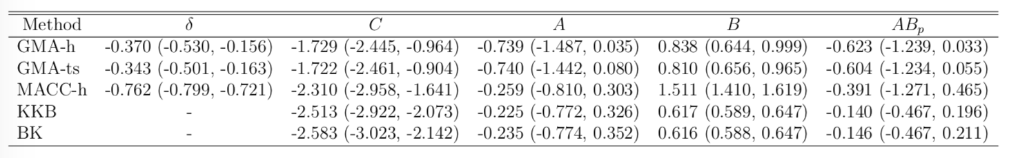
- STOP deactivates M1 directly ($C$) and indirectly ($AB$)
- preSMA mediates a good portion of the total effect
- Help resolve the debates among neuroscientists
- Other methods under-estiamte the effects
- Novel feedback findings: M1 → preSMA after lag 1 and 2 (not shown)
Discussion
- Mediation analysis for multiple time series
- Method: Granger causality + mediation
- Optimizing complex likelihood
- Theory: identifiability, consistency
- Result: low bias and improved accuracy
- Extension: functional mediation
- Paper in Biometrics 2019
- CRAN pkg:
gma and references within
Covariate Assisted Principal regression
Co-Authors
Yi Zhao
Indiana Univ Biostat

Bingkai Wang
Johns Hopkins Biostat
Johns Hopkins Medicine

Brian Caffo
Johns Hopkins Biostat
Statistics/Data Science Focuses
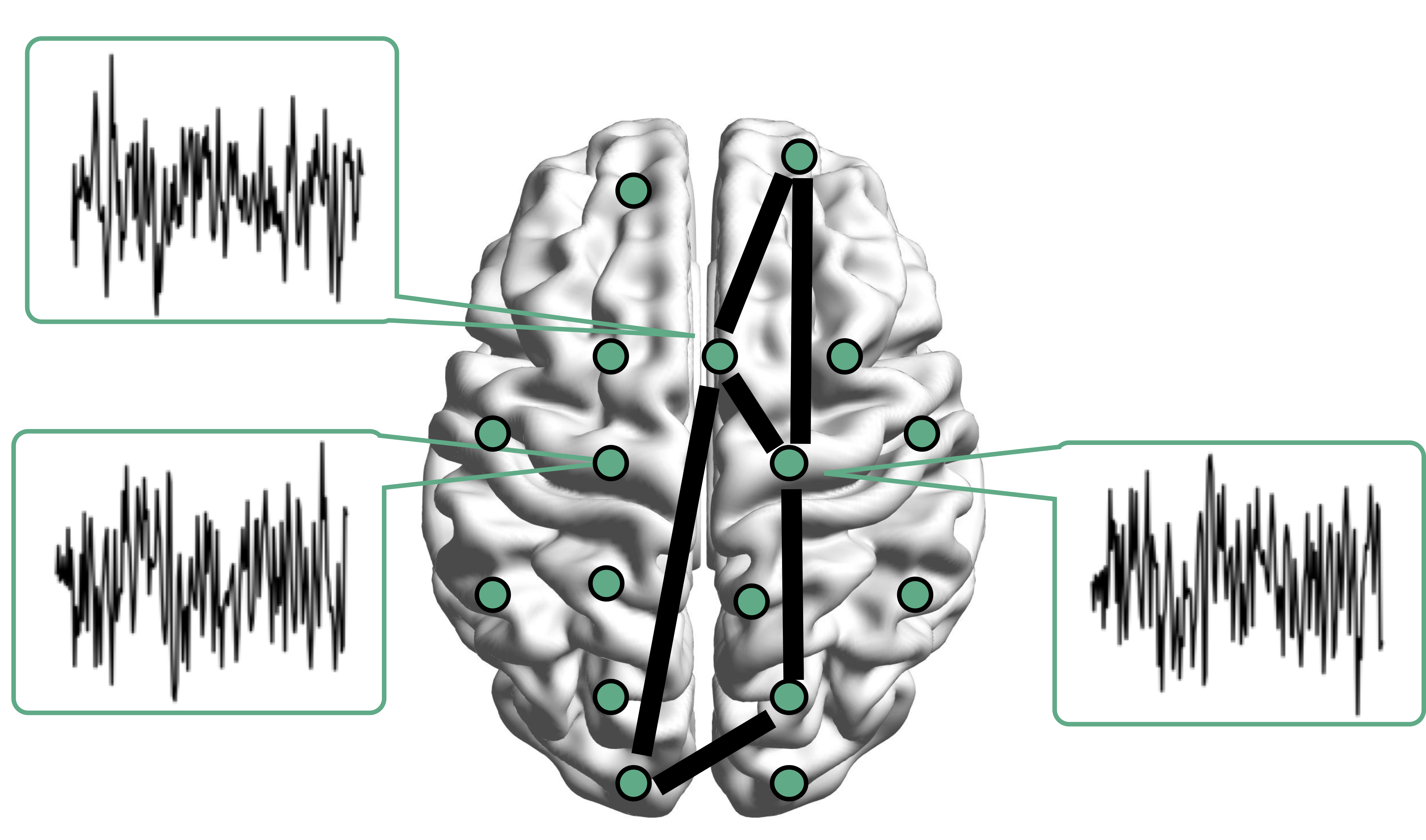
Motivating Example

Brain network connections vary by covariates (e.g. age/sex)
Resting-state fMRI Networks
- fMRI measures brain activities over time
- Resting-state: "do nothing" during scanning
- Brain networks constructed using
cov/cor matrices of time series
Mathematical Problem
- Given $n$ (semi-)positive matrix outcomes, $\Sigma_i\in \real^{p\times p}$
- Given $n$ corresponding vector covariates, $x_i \in \real^{q}$
- Find function $g(\Sigma_i) = x_i \beta$, $i=1,\dotsc, n$
- In essense,
regress positive matrices on vectors
Some Related Problems
- Heterogeneous regression or weighted LS:
- Usually for scalar variance $\sigma_i$, find $g(\sigma_i) = f(x_i)$
- Goal: to improve efficiency, not to interpret $x_i \beta$
- Covariance models Anderson, 73; Pourahmadi, 99; Hoff, Niu, 12; Fox, Dunson, 15; Zou, 17
- Model $\Sigma_i = g(x_i)$, sometimes $n=i=1$
- Goal: better models for $\Sigma_i$
- Multi-group PCA Flury, 84, 88; Boik 02; Hoff 09; Franks, Hoff, 16
- No regression model, cannot handle vector $x_i$
- Goal: find common/uncommon parts of multiple $\Sigma_i$
- Tensor-on-scalar regression Li, Zhang, 17; Sun, Li, 17
- No guarantees for positive matrix outcomes
Massive Edgewise Regressions
- Intuitive method by mostly neuroscientists
- Try $g_{j,k}(\Sigma_i) = \Sigma_{i}[j,k] = x_i \beta$
- Repeat for all $(j,k) \in \{1,\dotsc, p\}^2$ pairs
- Essentially $O(p^2)$ regressions for each connection
- Limitations: multiple testing $O(p^2)$, failure to accout for dependencies between regressions
Our CAP in a Nutshell
$\mbox{PCA}(\Sigma_i) = x_i \beta$
- Essentially, we aim to turn unsupervised PCA to a supervised PCA
- Ours differs from existing PCA methods:
- Supervised PCA Bair et al, 06 models
scalar-on-vector
- Supervised PCA Bair et al, 06 models
Model and Method
Model
- Find principal direction (PD) $\gamma \in \real^p$, such that: $$ \log({\gamma}^\top\Sigma_{i}{\gamma})=\beta_{0}+x_{i}^\top{\beta}_{1}, \quad i =1,\dotsc, n$$
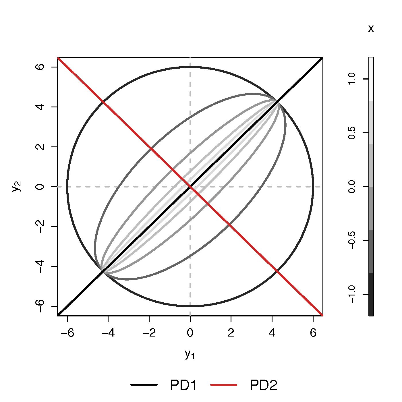
Example (p=2): PD1 largest variation but not related to $x$
PCA selects PD1, Ours selects
Advantages
- Scalability: potentially for $p \sim 10^6$ or larger
- Interpretation: covariate assisted PCA
- Turn
unsupervised PCA intosupervised
- Turn
- Sensitivity: target those covariate-related variations
Covariate assisted SVD?
- Applicability: other big data problems besides fMRI
Method
- MLE with constraints: $$\scriptsize \begin{eqnarray}\label{eq:obj_func} \underset{\boldsymbol{\beta},\boldsymbol{\gamma}}{\text{minimize}} && \ell(\boldsymbol{\beta},\boldsymbol{\gamma}) := \frac{1}{2}\sum_{i=1}^{n}(x_{i}^\top\boldsymbol{\beta}) \cdot T_{i} +\frac{1}{2}\sum_{i=1}^{n}\boldsymbol{\gamma}^\top \Sigma_{i}\boldsymbol{\gamma} \cdot \exp(-x_{i}^\top\boldsymbol{\beta}) , \nonumber \\ \text{such that} && \boldsymbol{\gamma}^\top H \boldsymbol{\gamma}=1 \end{eqnarray}$$
- Two obvious constriants:
- C1: $H = I$
- C2: $H = n^{-1} (\Sigma_1 + \cdots + \Sigma_n) $
Choice of $H$
Will focus on the constraint (C2)
Algoirthm
- Iteratively update $\beta$ and then $\gamma$
- Prove explicit updates
- Extension to multiple $\gamma$:
- After finding $\gamma^{(1)}$, we will update $\Sigma_i$ by removing its effect
- Search for the next PD $\gamma^{(k)}$, $k=2, \dotsc$
- Impose the orthogonal constraints such that $\gamma^{k}$ is orthogonal to all $\gamma^{(t)}$ for $t\lt k$
Theory for $\beta$
Theory for $\gamma$
Simulations
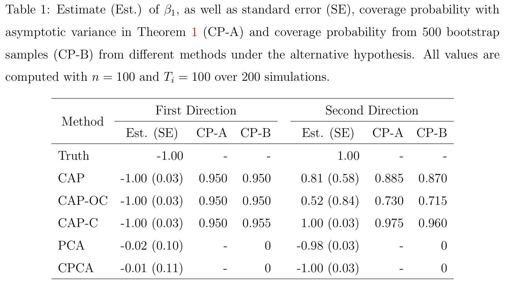
PCA and common PCA do not find the first principal direction, because they don't model covariates
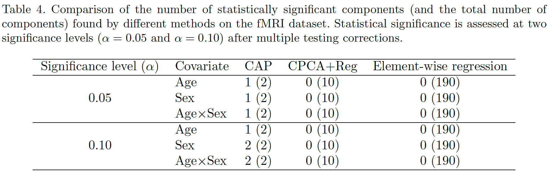
Resting-state fMRI
Regression Coefficients
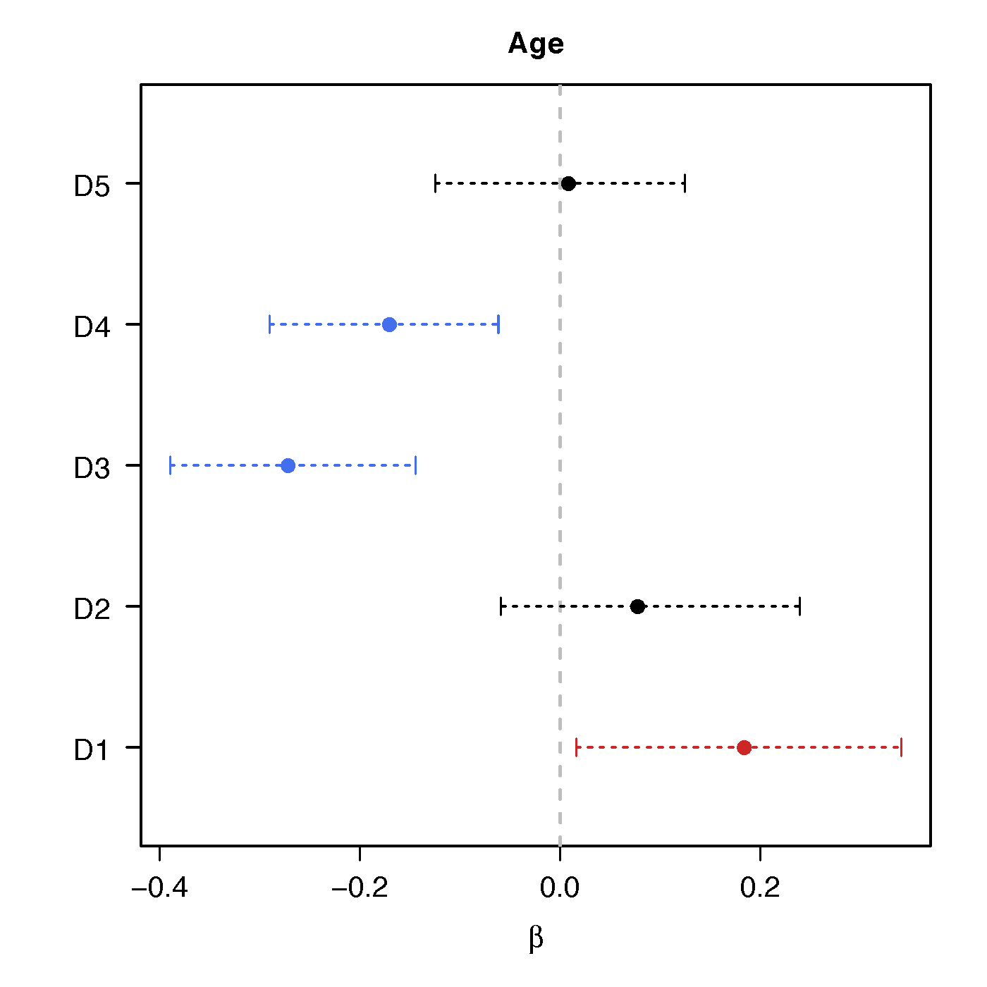
Age
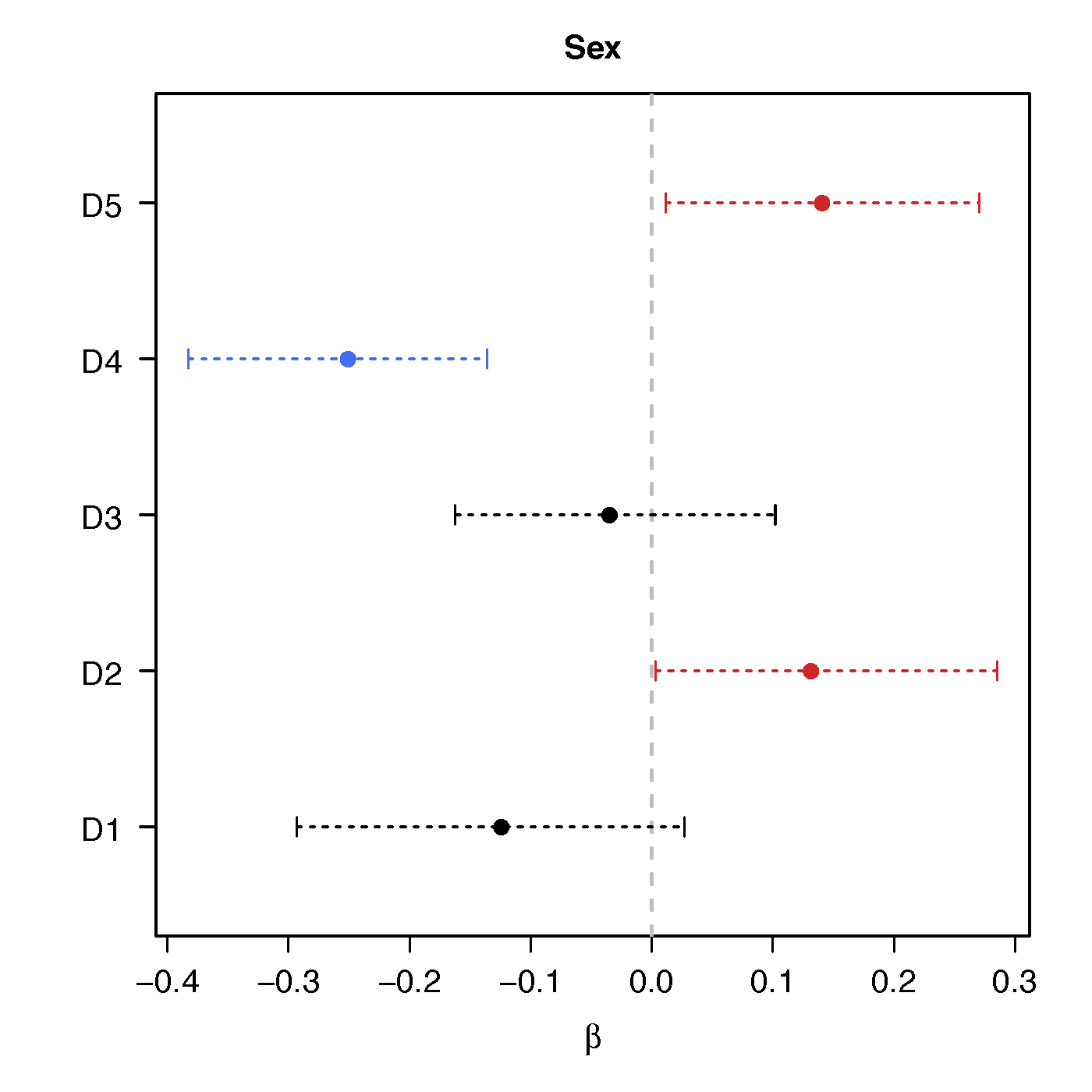
Sex
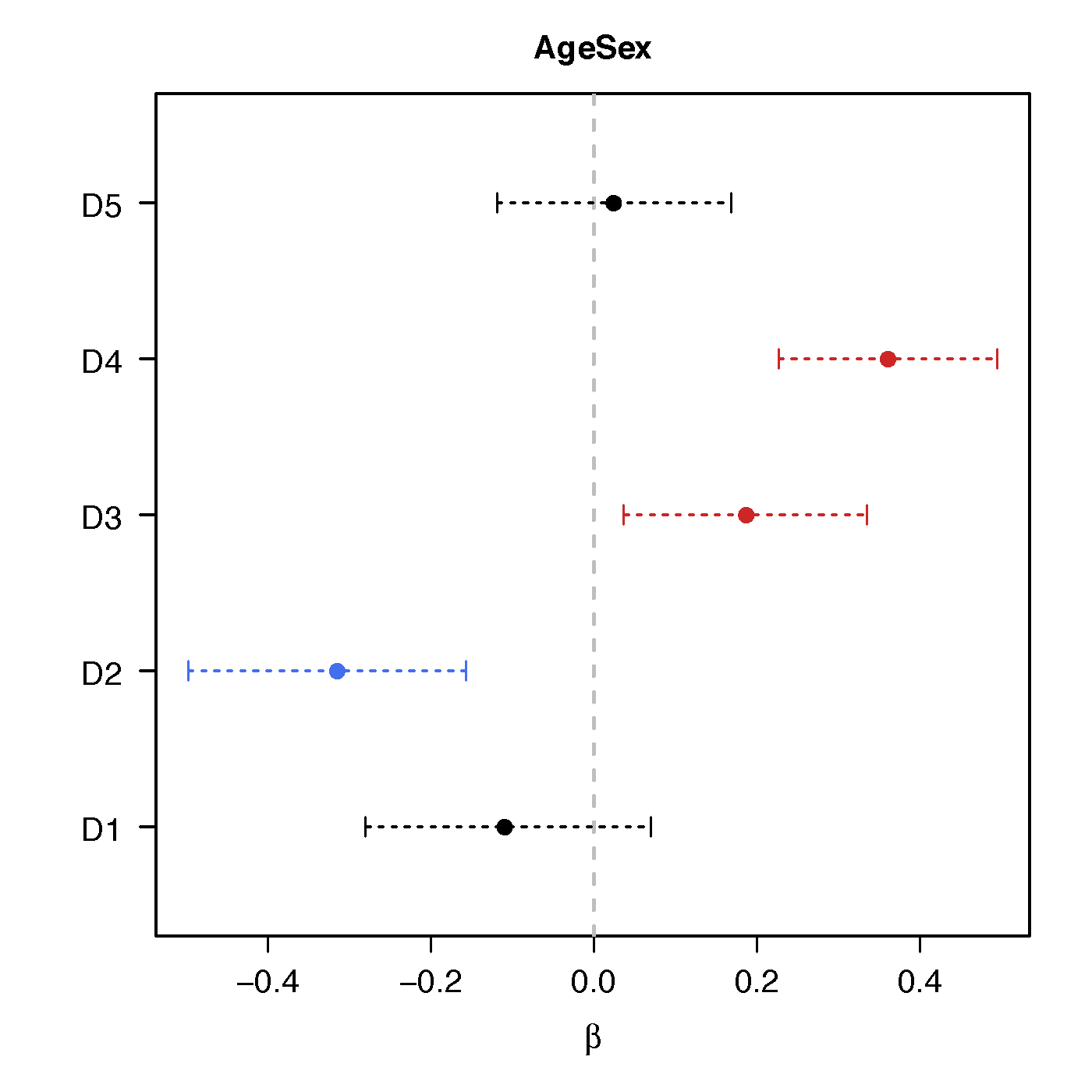
Age*Sex
No statistical significant changes were found by massive edgewise regression
Statistical Power
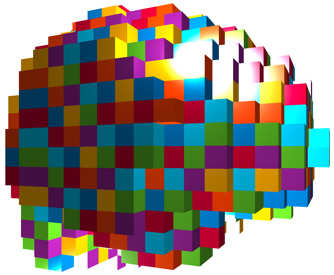
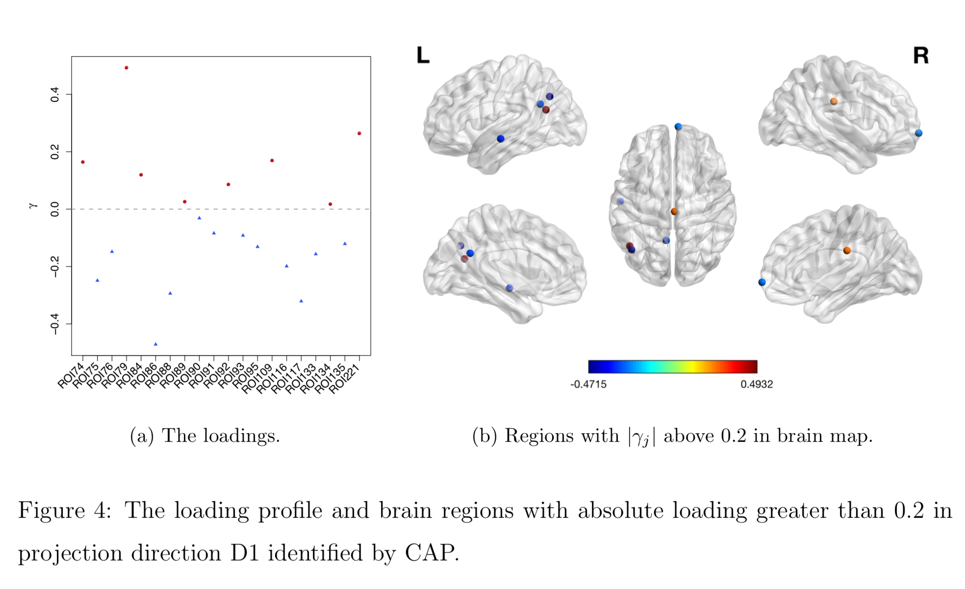
Brain Map of $\gamma$
Discussion
- Regress matrices on vectors
- Method to identify covariate-related directions
- Theorectical justification
- Manuscript: DOI: 10.1101/425033 (Revision for Biostatistics)
- R pkg:
cap 
Thank you!
Comments? Questions?
BigComplexData.com
or BrainDataScience.com