Variable Clustering via $G$-Models of Large Covariance Matrices
Xi (Rossi) Luo
Department of Biostatistics
Center for Statistical Sciences
Computation in Brain and Mind
Brown Institute for Brain Science
ABCD Research Group
December 20, 2016
Funding: NIH R01EB022911; NSF/DMS (BD2K) 1557467; NIH P20GM103645, P01AA019072, P30AI042853; AHA
Collaborators

Florentina Bunea
Cornell University

Christophe Giraud
Paris Sud University
Big Data Problem
- We are interested in
big cov with many variables-
Global property for certainjoint distributions - Real-world cov: maybe
non-sparse and other structures
-
- Clustering successful for Big Data Science Donoho, 2015
- Exploratory Data Analysis (EDA)Tukey, 1977
- Hierarchical clustering and KmeansHartigan & Wong, 1979
- Mostly based on
marginal/pairwise distances
- Can we combine clustering and big cov estimation?
Example: SP 100 Data
- Daily returns from stocks in SP 100
- Stocks listed in Standard & Poor 100 Indexas of March 21, 2014
- between January 1, 2006 to December 31, 2008
- Each stock is a variable
- Cov/Cor matrices (Pearson's or Kendall's tau)
-
Re-order stocks by clusters - Compare cov patterns with different clustering/ordering
-
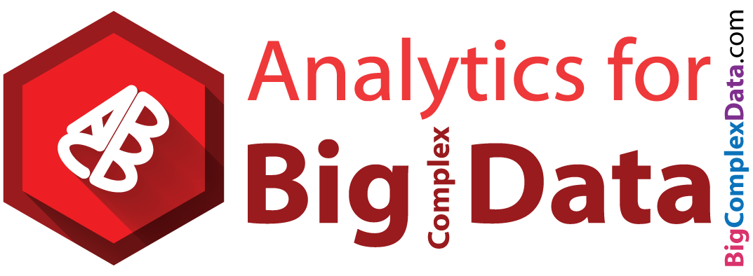
Cor after Grouping by Clusters
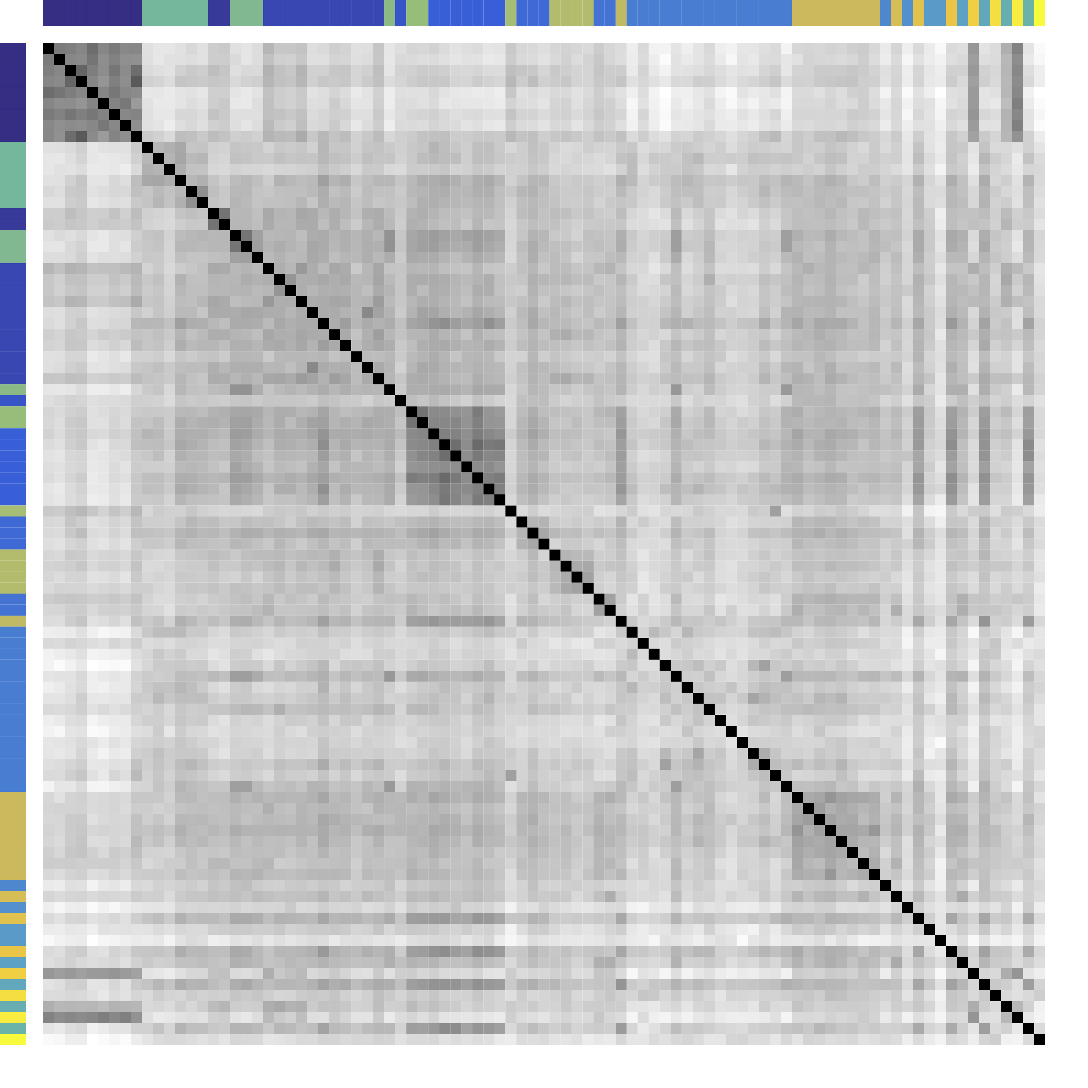
Ours yields stronger
Color bars: variable groups/clusters
Off-diagonal: correlations across clusters
Clustering Results
| Industry |
|
Kmeans | Hierarchical Clustering |
|---|---|---|---|
| Home Improvement | Home Depot, Lowe’s | Home Depot, Lowe’s, Starbucks, Target | Home Depot, Lowe’s, Starbucks, Target, Costco, Target, Wal-Mart, FedEx, United Parcel Service, Nike, McDonald’s |
| Telecom | ATT, Verizon | ATT, Verizon, Exelon, Comcast, Walt Disney, Time Warner | ATT, Verizon, Comcast, Walt Disney, Time Warner, AIG, Allstate, Metlife, American Express, Bank of America, Citigroup, US Bancorp, Wells Fargo, Capital One, Goldman Sachs, JP Morgan Chase, Morgan Stanley, Simon Property, General Electric |
| Diversified Metals & Mining | Freeport-McMoran | Freeport-McMoran, National Oillwell Varco | Freeport-McMoran, Apache Corp., Anadarko Petroleum, Devon Energy, Halliburton, National Oillwell Varco, Occidental Petroleum, Schlumberger, ConocoPhillips, Chevron, Exxon |
| $\cdots$ | |||
Model
Problem
- Let ${X} \in \real^p$ be a zero mean random vector
- In certain problems, means are arbitrary
- Divide variables into partitions/clusters
- Example: $\{ \{X_1, X_3, X_7\}, \{X_2, X_5\}, \dotsc \}$
- Theoretical: Find a partition $G = \{G_k\}_{ 1 \leq k \leq K}$ of $\{1, \ldots, p\}$ such that all $X_a$ with $a \in G_k$ are
"similar" - Big Data:
"helpful" clustering that shows patterns
Related Areas
- Clustering: Kmeans and Hierarchical Clustering
- Usually for clustering
$n$ observations in $R^p$ - Advantages: fast, general, popular
- Limitations: low signal-noise-ratio, theory, NP-hard
- Q: How to choose number of clusters? Theory?
- Q: Can clusters contain singletons?
- Usually for clustering
- Community detection: huge literature see review Newman, 2003 but start with
observed adjacency matrices or networks- Ours for data that can be generated from
unknown networks
- Ours for data that can be generated from
- These are related but different problems
Model: Starting Point
$$ X_{n\times p}=\underbrace{Z_{n\times k}}_\text{Source/Factor} \quad \underbrace{G_{k\times p}}_\text{Mixing/Loading} + \underbrace{E_{n\times p}}_{Error} \qquad Z \bot E$$
- Clustering: $G$ is $0/1$ matrix for $k$ clusters/ROIs
- Decomposition:
- PCA/factor analysis: orthogonality
- ICA: orthogonality → independence
- matrix decomposition: e.g. non-negativity
- This model leads to
block patterns in $\cov(X)$- $\cov(X) = G^T \cov(Z) G + \cov(E)$
- Note: not necessarily block-diagonal
Generalization: $G$-Block
- Example: $G=\ac{\ac{1,2};\ac{3,4,5}}$, $X \in \real^p$ is $G$-block
$$\Sigma =\left(\begin{array}{ccccc} {\color{red} D_1} & {\color{red} C_{11} }&C_{12} & C_{12}& C_{12}\\ {\color{red} C_{11} }&{\color{red} D_1 }& C_{12} & C_{12}& C_{12} \\ C_{12} & C_{12} &{\color{green} D_{2}} & {\color{green} C_{22}}& {\color{green} C_{22}}\\ C_{12} & C_{12} &{\color{green} C_{22}} &{\color{green} D_2}&{\color{green} C_{22}}\\ C_{12} & C_{12} &{\color{green} C_{22}} &{\color{green} C_{22}}&{\color{green} D_2} \end{array}\right) \qquad C = \left(\begin{array}{cc} {\color{red} C_{11} } & C_{12}\\ C_{12} & {\color{green} C_{22}} \end{array}\right) $$ - Matrix math: $\cov(X) = \Sigma = G^TCG + d$
- We allow $|C_{11} | \lt | C_{12} |$ or
$C \prec 0$ - Kmeans/HC leads to block-diagonal cor matrices (permutation)
- Clustering based on $G$-Block
- From $G$-block we can read out
"negative" $\cov(Z)$ - Cov defined for semiparametric distributions
- Clusters can contain singletons
- From $G$-block we can read out
Minimum $G$ Partition
- We define the minimal cluster/partition.
- The minimal partition is unique under conditions.
- We will aim to recover the minimal partition (thus $K$).
Method
New Metric: CORD
- First, pairwise correlation distance (like Kmeans)
- Gaussian copula: $$Y:=(h_1(X_1),\dotsc,h_p(X_p)) \sim N(0,R)$$
- Let $R$ be the correlation matrix
- Gaussian: Pearson's
- Gaussian copula: Kendall's tau transformed, $R_{ab} = \sin (\frac{\pi}{2}\tau_{ab})$
Algorithm: Main Idea
- Greedy: one cluster at a time, avoiding NP-hard
- Cluster variables together if CORD metric $$\widehat \d(a,b) \lt \alpha$$ where $\alpha$ is a tuning parameter
- $\alpha$ is chosen by theory or CV
Theory
Condition
The signal strength $\eta$ is large.
Consistency
Ours recovers the exact clustering with high probability.
Minimax
Group separation condition on $\eta$ is optimal.
Choosing Number of Clusters
- Split data into 3 parts
- Use part 1 of data to estimate clusters $\hat{G}$ for each $\alpha$
- Use part 2 to compute between variable difference $$ \delta^{(2)}_{ab} = R_{ac}^{(2)} - R_{bc}^{(2)}, \quad c \ne a, b. $$
- Use part 3 to generate "CV" loss $$ \mbox{CV}(\hat{G}) = \sum_{a \lt b} \| \delta^{(3)}_{ab} - \delta^{(2)}_{ab} 1\{ a \mbox{ not clustered w/ } b \} \|^2_\infty. $$
- Pick $\alpha$ with the smallest loss above
Theory for CV
Simulations
Setup
- Model $C$ ($\cov(Z)$): positive semidefinite or negative
- True $G^*$: singletons or no-singleton clusters
- Simulate $X$ from $G$-block cov
- Variable clustering using $X$
- Compare with K-means or Hierarchical Clustering:
- Exact recovery of groups
- Cross validation loss and choosing $K$
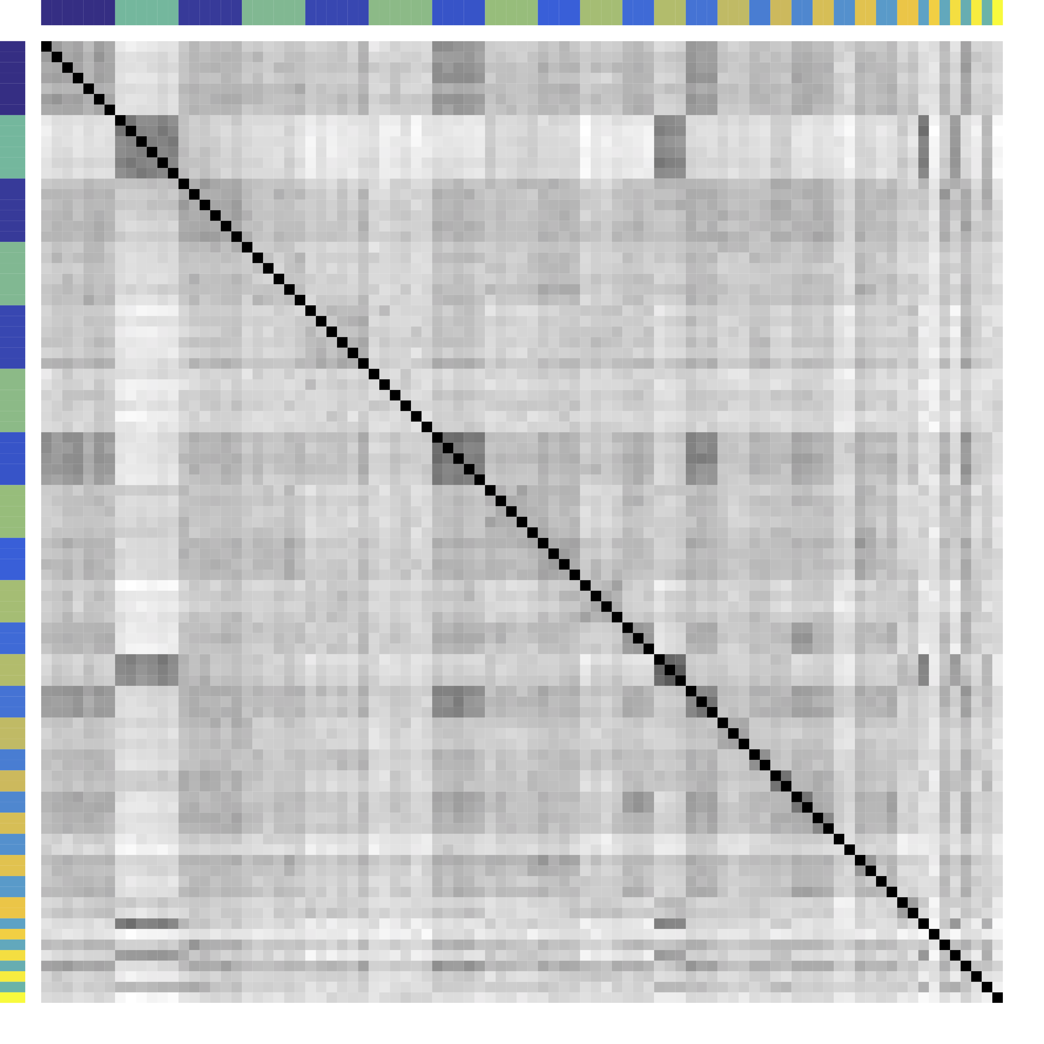
Exact Recovery
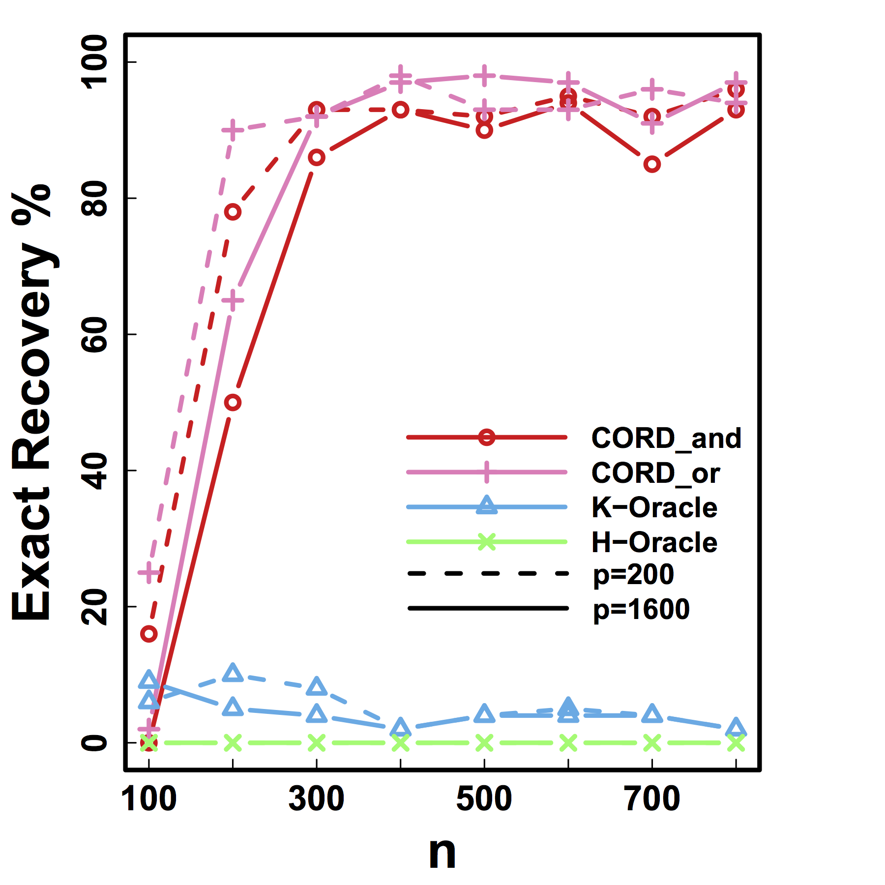
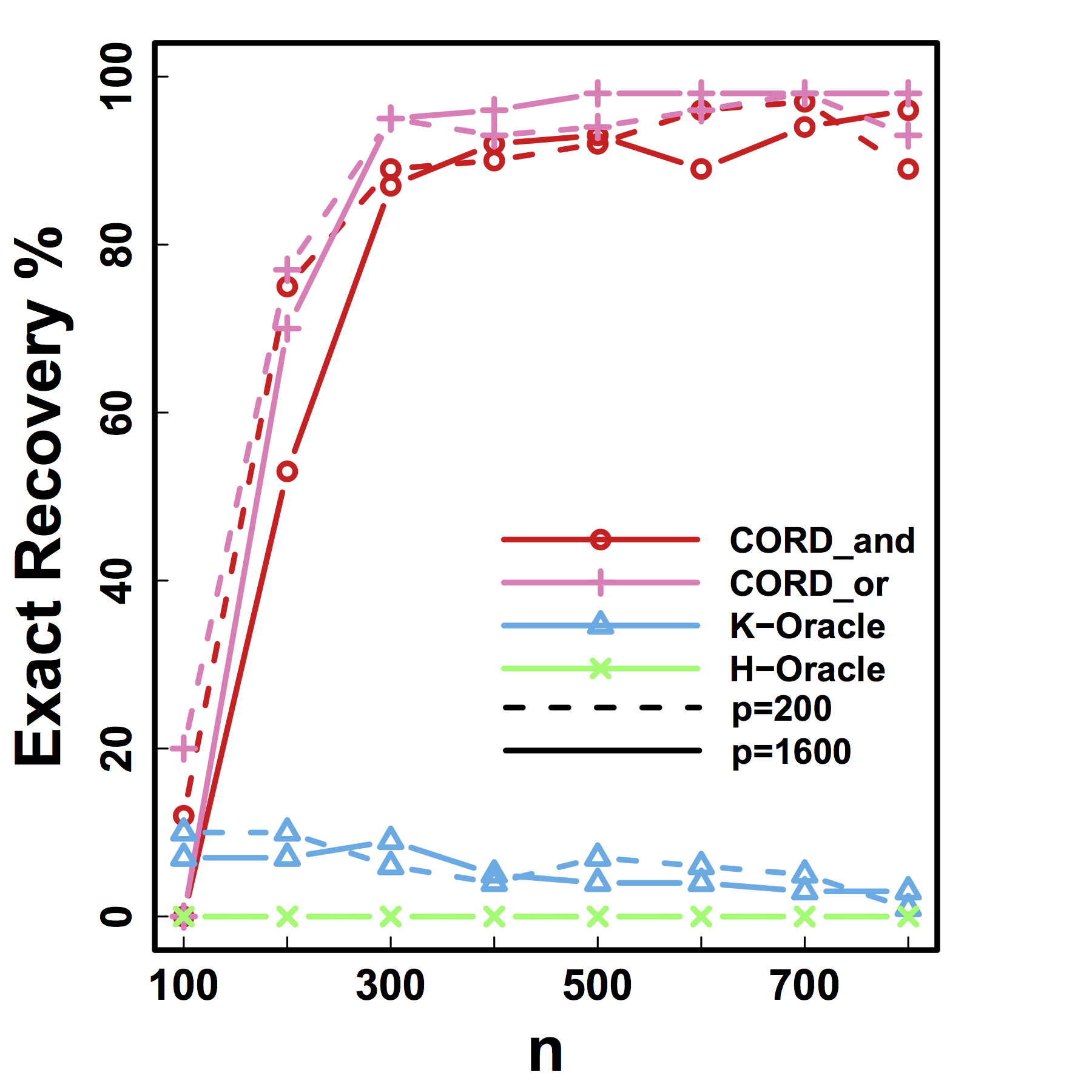
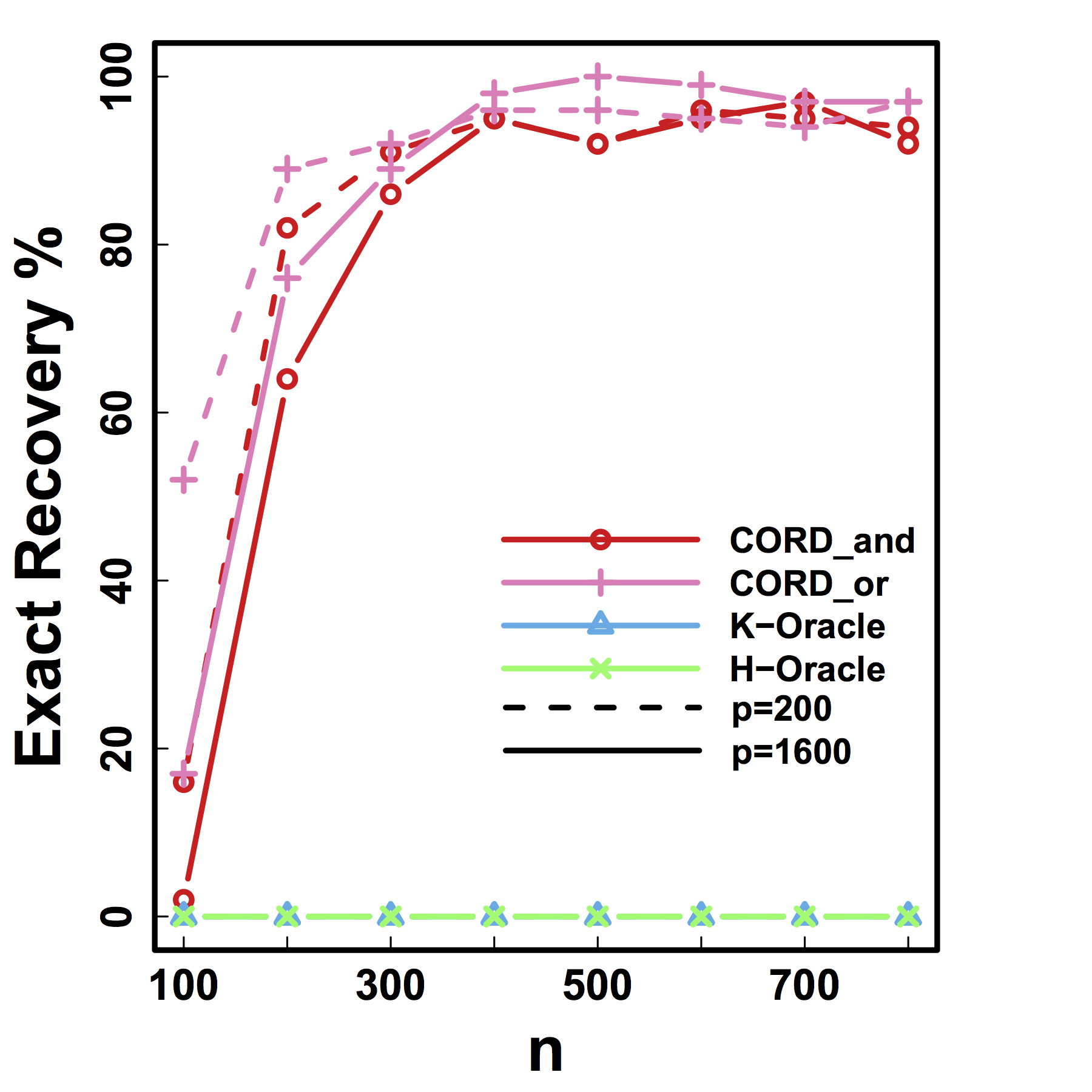
Different models for $C$="$\cov(Z)$" and $G$
HC and Kmeans fail even if inputting the true $K$ and $n \rightarrow \infty$
Our CORD methods recover both the true $G^*$ and $K$ as predicted by our theory.
Cross Validation

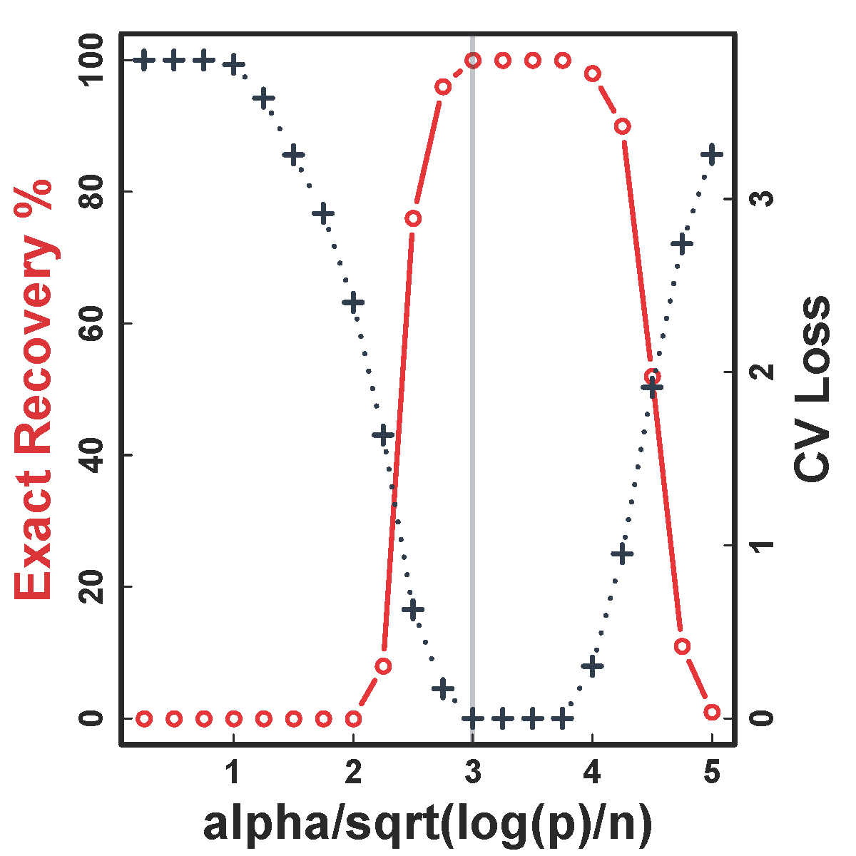
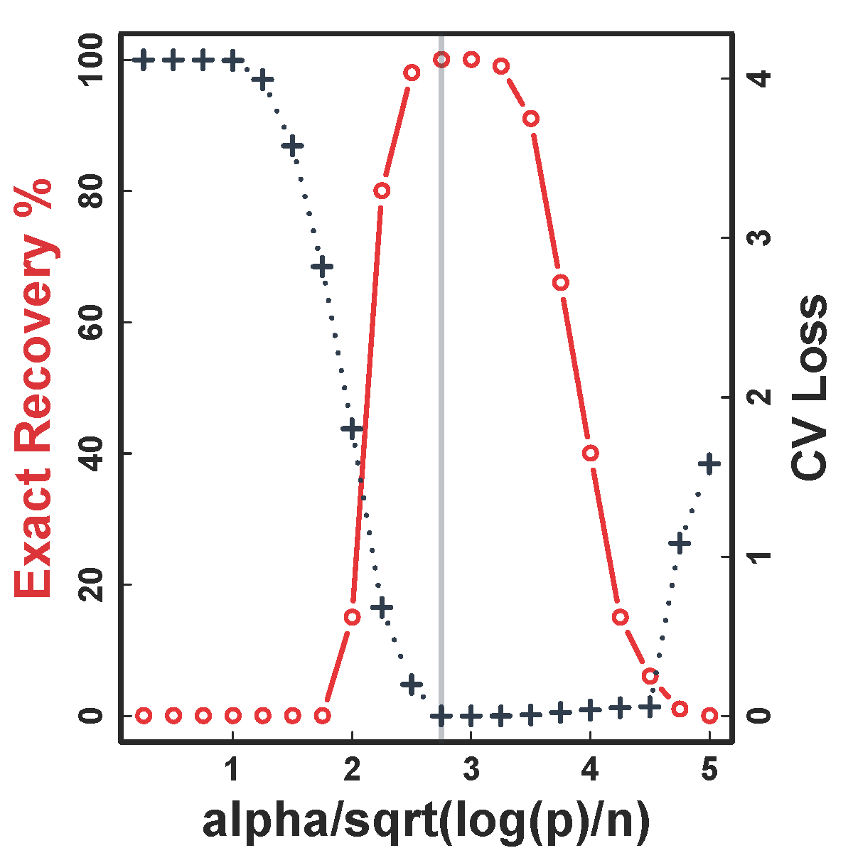
CV selects the constants to yield close to 100% recovery, as predicted by our theory (at least for large $n>200$)
Real Data
Functional MRI
- fMRI matrix: BOLD from different brain regions
- Variable: different brain regions
- Sample: time series (after whitening or removing temporal correlations)
-
Clusters of brain regions
- Two data matrices from two scan sessions OpenfMRI.org
- Use Power's 264 regions/nodes
Test Prediction/Reproducibilty
- Find partitions using the first session data
- Average each block cor to improve estimation
- Compare with the cor matrix from the second scan $$ \| Avg_{\hat{G}}(\hat{\Sigma}_1) - \hat{\Sigma}_2 \|$$
- Difference is smaller if clustering $\hat{G}$ is better
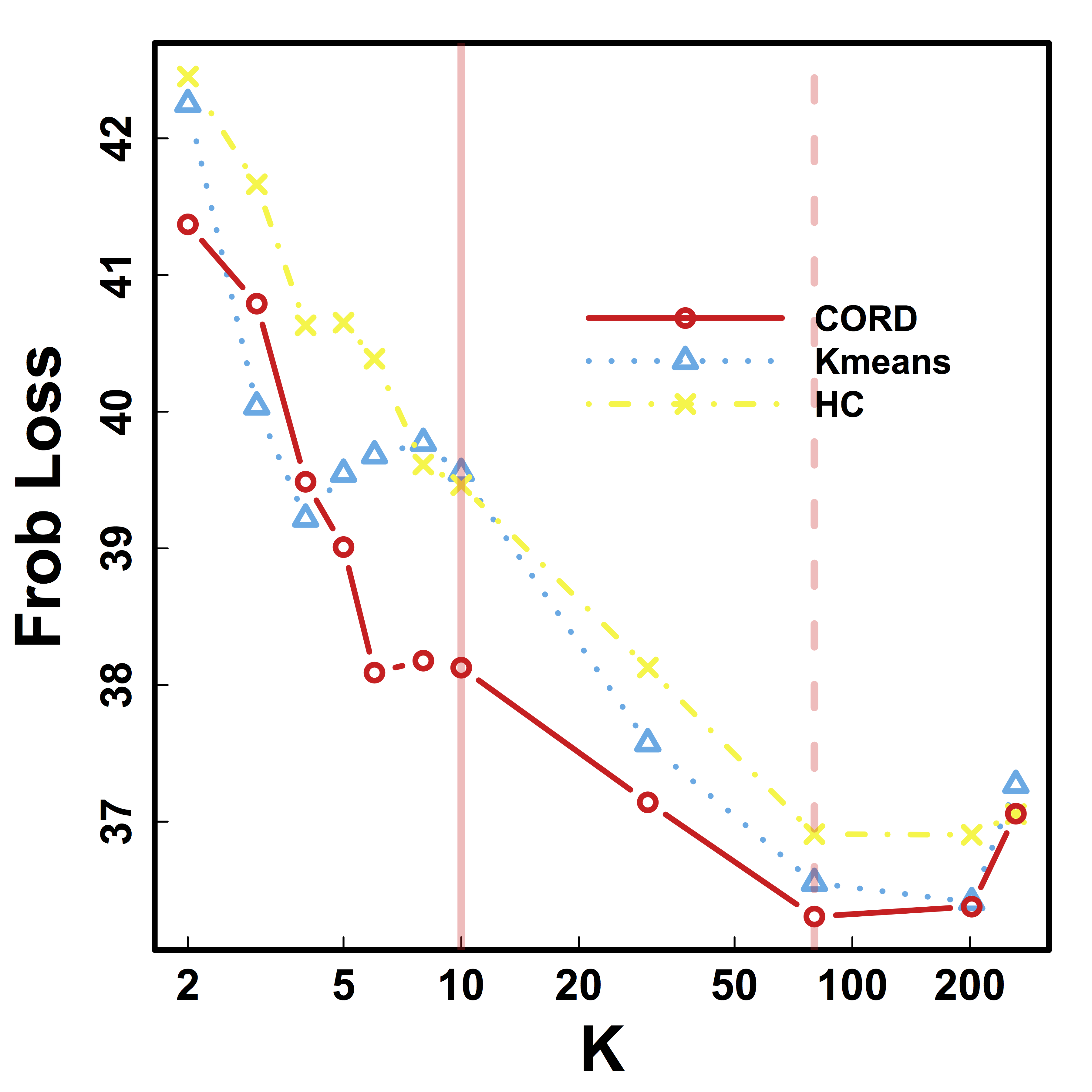
Vertical lines: fixed (solid) and data-driven (dashed) thresholds
Our CORD $\hat{G}$ leads to smaller between-session variability for almost all $K$, than HC and Kmeans.
Discussion
- Cov + clustering:
- Identifiability, accuracy, optimality
- $G$-models: $G$-latent, $G$-block, $G$-exchangeable
- New metric, method, and theory
- Defining clusters, consistency, minimax, and CV theory
- Some new results using big data examples
- Paper:
bit.ly/cordCluster (arXiv 1508.01939) - R package:
cord on CRAN- CV function available soon
Thank you!
Slides at: bit.ly/ICSA2016

Website: Big Complex Data.com
Postdoc position available
funded by Whitehouse's Big Data and BRAIN Initiatives